The magic in AI and Machine Learning

Before beginning, I'd like to shout out to Hala Nelson and her new book Essential Math for AI for inspiring this post. I wish I had this book while taking some of my classes at Georgia Tech!
“Magic” and AI Hype
If you spend any time on LinkedIn, you probably know that the hype around AI, LLMs, and GenAI is entirely off the charts; take a peek at any of the prominent enterprise IT vendors other than NVIDIA, and you'll find a lot of marketing materials around their newly discovered AI solutions. There is a feeling that a gold rush is happening among enterprise IT organizations scrambling to catch the latest AI wave. Just sprinkle some AI magic onto your product and profit!
On the flip side, there seems to be some dark, magical thinking around AI causing harm to humanity or, worse, possibly destroying the human race. Yann LeCun has stated that some of the existential angst around AI destroying humanity is "preposterously ridiculous", and Andrew Ng has stated his "greatest fear for the future of AI is if overhyped risks" is that "tech lobbyists get enacted stifling regulations that suppress open-source and crush innovation."
While some of my comments about the current wave of AI hype may sound a bit cynical and make it seem that the hype is at the two extremes of a Gaussian distribution, I think there's good reason for excitement and believe that the "magic" of AI can solve real-world problems.
What is this "magic" that can solve real-world problems?
MATH!
I may sound cliche and a bit like your junior high math teacher, but math is everywhere and can help us solve many complex, real-world problems.
For this post, I want to talk about the math behind linear regression.
What?! Boo!!
Why are we talking about linear regression?!
It's old, boring, and definitely not as sexy as some of the latest advancements in machine learning and AI.
Yeah, well… Linear regression is a good place to start to get at the heart of machine learning and AI. But what is it that's at the heart of AI?
It's optimization!
Optimization is at the heart of machine learning and deep learning algorithms and linear regression is a nice, simple place to help us begin to get our heads around this concept.
What is optimization?
The field of optimization is a branch of mathematics and computer science that deals with finding the best possible solution to a problem from a set of feasible solutions. Many disciplines involve optimization at their core. For example, in physics, systems are driven to their lowest energy state subject to physical laws, whereas in business, corporations aim to maximize shareholder value. In aviation, airlines might select a flight plan for an aircraft to minimize time or fuel use.
Optimization aims to minimize or maximize an objective function subject to a set of constraints. The objective function represents the parameter to be optimized, while the constraints define the acceptable solutions. Optimal solutions are those that satisfy the constraints and either minimize or maximize the objective function.
In machine learning and deep learning, when we train our models, optimization is a fundamental step where the algorithm adjusts the model parameters to minimize a predefined loss function. Optimization is also used to find a model's optimal set of hyperparameters. For example, in neural networks, we might use stochastic gradient descent during training to optimize the weights and biases of the network during the training process.
Least Squares Estimation
With that in mind, let's dig into our simple linear regression example and see how optimization plays a role.
If you've been living under a rock, linear regression is a statistical method used to model the relationship between a dependent variable and one or more independent variables. It assumes that there is a linear relationship between the variables, meaning that a change in the independent variable(s) is associated with a proportional change in the dependent variable.
For simple linear regression, we have the form:
In the case of multiple linear regression, we have:
Given our linear regression training functions, we can employ a bit of linear algebra to rewrite these equations in matrix form:
where
Note that each row in X (the design matrix) represents an observation and that our design matrix has been augmented with a vector of ones which will help us find the y-intercept (𝛽0) when we estimate our 𝛽 coefficients.
The question you should be asking is: Given a set of observations, X, and our training function,
how do we go about estimating our 𝛽 coefficients?
To help us find our 𝛽 coefficients, we need to define a loss function. This is where the magic comes in!
In mathematics, we can choose how to construct a loss function (or error function).
What's a loss function?
In machine learning (and statistics), a loss function is a mathematical function that measures the difference between the predicted values generated by a model and the actual values (ground truth) of the target variable. The goal during the training of our model is to minimize this loss function such that the model is optimized to make predictions that are as close as possible to the actual values.
Typically, with ordinary least squares (OLS) regression, this means we want to minimize the squared error (or mean squared error). We could use another loss function, such as absolute error (or mean absolute error), but we run into the problem of the function not being differentiable at certain points, i.e.) f(x)=|x| is not differentiable at x=0.
For this example, let's use the mean squared error:
Substituting in our training function from above, we get:
Now that we've decided on a loss (or objective) function, we can restate it as an optimization problem:
To find our 𝛽 estimates, we simply need to minimize our loss function with respect to 𝛽. Since our loss function is continuous and convex, we can simply take the derivative, set it to zero, and solve for 𝛽 to get our 𝛽 estimates.
Note here that 𝛽-hat (the 𝛽 with the little hat) is our estimated 𝛽 coefficients. These are the estimates for our best-fit regression line.
Let's go ahead and define our loss function as:
To make our derivation easier, let's expand our loss function:
Note that we can use the following identity to combine terms in our loss function:
To find our 𝛽-hat estimates, we can simply take the derivative with respect to 𝛽:
To help with the derivation, take note that:
Which, in our case, leads us to
Next, let's set our derivative equal to zero and solve for 𝛽-hat:
Eliminating the -2, 1/n, and transposing, we get a closed-form solution (the normal equation):
Finally, we can isolate 𝛽-hat to get:
Now that we have 𝛽-hat, let's put this into practice to see how this works with some code.
First, let's start with the case of simple linear regression.
First make sure you have all your imports:
import numpy as np
import pandas as pd
import matplotlib.pyplot as plt

from sklearn.datasets import make_regression
from sklearn.linear_model import LinearRegression

from typing import List, Dict
from numpy.typing import NDArray
Next, let’s define a simple linear function:
def simple_line_func(x: NDArray, B0: float, B1: float) -> NDArray:
    # y = B1*x + B0
    assert type(x) == list or type(x) == np.ndarray
    return x*B1 + B0
Next, let’s generate some fake data with our simple linear function and add in some random noise from a Gaussian distribution (variable y1). Let’s also augment the X data with a column of 1s; this will help identify the y-intercept (𝛽0) estimate.
np.random.seed(42)
n = 10
steps = 500
X = np.linspace(1,n, steps)
y = simple_line_func(X, 2, 3)
y1 = y + np.random.normal(loc=0.0, scale=2.0, size=steps)
X_aug = np.concatenate([[np.ones(steps)],[X]], axis=0).T
To fit our data, we can simply use our equation from above:
This is what that equation looks like in code:
betas = np.linalg.inv(X_aug.T@X_aug)@X_aug.T@y1When we print the contents of our betas variable, we get the following:
array([1.92335698, 3.01642164])Note that the first value is pretty close to what we specified as the y-intercept (2: simple_line_func(X, 2, 3). Also, notice how the second value is very close to what we specified as 𝛽1 (3).
To verify the results of our 𝛽-hat estimates, lets double check against the sklearn linear regression implementation:
reg = LinearRegression().fit(X.reshape(-1,1), y)
print(f"B0: {reg.intercept_}")
print(f"B1: {reg.coef_[0]}")
When we pass in the original y values and unaugmented X values, we the same y-intercept and 𝛽1 values (2 and 3: simple_line_func(X, 2, 3)).
B0: 1.9999999999999964
B1: 3.0000000000000004
Next when we fit the sklearn model with the noisy y values, we get the same y-intercept and 𝛽1 estimate as our equation from above:
reg = LinearRegression().fit(X.reshape(-1,1), y1)
print(f"B0: {reg.intercept_}")
print(f"B1: {reg.coef_[0]}")
B0: 1.9233569778162867
B1: 3.0164216384292746To visualize what we are doing, let’s plot this out. The green line is our true y values, and the dashed red line is the fitted line based on the 𝛽 estimates we found from our equation. Note how the green and red dashed lines are practically the same. That makes sense since the 𝛽 estimates are very close to the original 𝛽s. (1.92335698, 3.01642164 vs 2 and 3)
y_pred = betas[1]*X + betas[0]

plt.scatter(X, y1, s=2, alpha=0.4)
plt.plot(X, y, 'green', alpha=0.8)
plt.plot(X, y_pred, 'r--', alpha=0.8)
plt.tight_layout()
plt.show()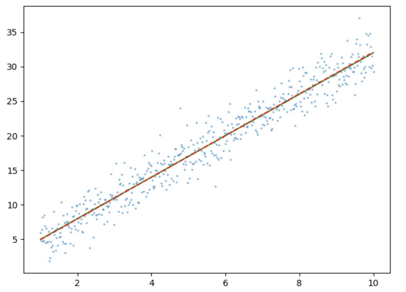
Finally, let’s see how the equation for the 𝛽 estimates works for multiple linear regression. I will use sklearn’s make_regression function to generate a dataset in this example.
np.random.seed(42)

n = 10
steps = 500

X, y = make_regression(n_samples=500, n_features=5, bias=np.pi)
ones = np.ones(steps).reshape(steps,1)
X_aug = np.append(ones, X,axis=1)
Let’s fit the model using our equation for the 𝛽 estimates:
betas = np.linalg.inv(X_aug.T@X_aug)@X_aug.T@y
print(f"Intercept: {np.round(betas[0], 6)}")
print(f"Beta Estimates: {np.round(betas[1:], 6)}")
Intercept: 3.141593
Beta Estimates: [68.513431 11.043186 30.980688 81.412569 28.918745]When we fit the model using sklearn we get:
reg = LinearRegression().fit(X, y)
print(f"Intercept: {reg.intercept_}")
print(f"Beta Estimates: {reg.coef_}")
Intercept: 3.141592653589795
Beta Estimates: [68.51343099 11.04318634 30.98068753 81.41256856 28.91874463]Look at that! Our y-intercepts and 𝛽 estimates are all essentially the same! As you can see, our method to estimate 𝛽 also works for multiple linear regression.
Conclusion
As we have seen, optimization is key to linear regression because the goal is to find the best-fitting line that minimizes the difference between the predicted and actual values in the training dataset (loss function). To help find the best-fitting line, we minimized our loss function (mean squared error) to find the estimated 𝛽 coefficients. Once we found our estimated 𝛽 coefficients, we were able to construct a function to predict new values and plot a best-fit line to our data. Finally, we verified (with comparisons to sklearn) that our method of finding our estimated 𝛽 coefficients works for both simple and multiple linear regression.