
Solving Linear Regression Problems Using PyTorch


Simple Linear Regression
In my last few posts, I discussed linear regression and how we find the beta estimates for ridge and lasso regression problems. In keeping with that theme and continuing my journey with PyTorch, I wanted to demonstrate how simple it is to build a linear model with PyTorch and then see how we can extend our model to handle more complex problems.
To help get things rolling, these are the imports that I’m using for this post:
import numpy as np
import matplotlib.pyplot as plt

import torch
import torch.nn as nn

from torcheval.metrics import R2Score, MeanSquaredError

from sklearn.datasets import make_regression
from sklearn.linear_model import LinearRegression
from sklearn.model_selection import train_test_split
from sklearn.metrics import mean_squared_error, r2_score
Next, let’s generate a simple linear dataset with one feature; we can use sklearn’s make_regression function to do that.
bias = 3.0
X, y, coef = make_regression(n_samples=1200, n_features=1, bias=bias, noise=2, random_state=42, shuffle=True, coef=True)
X_train, X_val, y_train, y_val = train_test_split(X[:1000], y[:1000], test_size=0.20, random_state=42, shuffle=True)
X_train = torch.tensor(X_train, dtype=torch.float)
X_val = torch.tensor(X_val, dtype=torch.float)
y_train = torch.tensor(y_train, dtype=torch.float).unsqueeze(dim=1)
y_val = torch.tensor(y_val, dtype=torch.float).unsqueeze(dim=1)
X_test, y_test = X[1000:], y[1000:]
X_test = torch.tensor(X_test, dtype=torch.float)
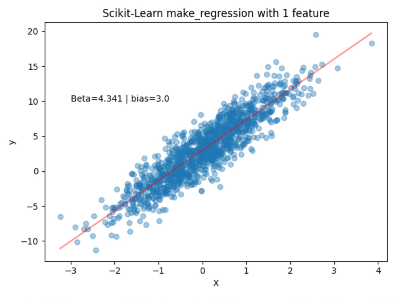
y_test = torch.tensor(y_test, dtype=torch.float).unsqueeze(dim=1)In the code snippet above, we generate 1200 data points with a bias of 3.0. When we look at the coef variable, we have a single coefficient of 4.341. Plotting the data points and overlaying the line (y = 4.341X + 3.0) we get the following:
Before building a PyTorch model, let’s first check how sklearn’s LinearRegression implementation performs with this data.
lr = LinearRegression()
lr.fit(X_train, y_train)
y_pred =  lr.predict(X_test)
r2_score(y_test, y_pred)
print(f"coef: {lr.coef_[0][0]}")
print(f"bias: {lr.intercept_[0]}")
print(f"R2: {r2_score(y_test, y_pred)}")
print(f"MSE: {mean_squared_error(y_test, y_pred)}")
coef: 4.38670539855957
bias: 3.0133330821990967
R2: 0.7943845110389801
MSE: 4.218380451202393
Fitting sklearn’s LinearRegression implementation to the training data and then calculating R2, we see that this model explains roughly 79.4% of the variance in the dependent variable, y, which can be explained by the independent variable X. Calculating the MSE, we get a score of ~ 4.22.
Great! Now we have a baseline to gauge our PyTorch model. We know that the true coefficient is 4.341, our bias is 3.0, and Sklearn’s linear regression implementation explains roughly 79.4% of the variability in the data and the fitted coefficient is ~4.3867, with a bias of ~3.0133.
So, how do we solve a simple linear regression problem with PyTorch? The key lies with the PyTorch’s Linear layer: Linear — PyTorch 2.2 documentation. PyTorch’s linear layer simply applies a linear transformation to the incoming data:
To use our PyTorch linear layer, we can create a class called simple_linear_model that inherits the nn.Module class. We use super().__init__() within our __init__() function to give us access to methods from the parent class from within a child class without having to refer to the parent class explicitly. Next, we can create an instance of nn.Linear() and call it self.linear. We can then use that linear layer in our models forward pass. To do that, we simply call self.linear() in the forward function and return the results.
class simple_linear_model(nn.Module):
    def __init__(self, in_features=1, out_features=1):
        super().__init__()
        self.linear = nn.Linear(in_features=in_features,
                                out_features=out_features)
    def forward(self, x):
        return self.linear(x)
The training loop for this model is listed below. We will use this training loop when we build a model for more complex problems. Note that we are using MSE loss and the Adam optimizer.
Additionally, to help with predictions and plotting the loss curves, we define a predict function and a loss plotting function.
def training_loop(model, X_train, y_train, X_val, y_val, epochs = 1000, seed=42, device='cpu'):
    torch.manual_seed(seed)

    train_loss_values = []
    val_loss_values = []
    epoch_count = []

    X_train = X_train.to(device)
    X_val = X_val.to(device)
    y_train = y_train.to(device)
    y_val = y_val.to(device)

    model = model.to(device)
    loss_fn = nn.MSELoss()
    optimizer = torch.optim.Adam(params=model.parameters(), lr=0.001)

    for epoch in range(epochs):
        ### Training
        model.train()
        y_pred = model(X_train)
        loss = loss_fn(y_pred, y_train)
        epoch_count.append(epoch)
        train_loss_values.append(loss.item())
        optimizer.zero_grad()
        loss.backward()
        optimizer.step()

        ### Validation
        model.eval()
        with torch.inference_mode(): #.no_grad():
          val_pred = model(X_val)
          val_loss = loss_fn(val_pred, y_val)
          val_loss_values.append(val_loss.item())
          if epoch % 1000 == 0:
                print(f"Epoch: {epoch} | Train Loss: {loss} | Validation Loss: {val_loss} ")
    return train_loss_values, val_loss_values, epoch_count


def predict(model, data, device='cpu'):
    model = model.to(device)
    model.eval()
    with torch.inference_mode(): #.no_grad():
        y_preds = model(X_test.to(device))
    return y_preds


def plot_losses(train_loss_values, val_loss_values, epoch_count):
    plt.plot(epoch_count, train_loss_values, label="Train loss")
    plt.plot(epoch_count, val_loss_values, label="Validation loss")
    plt.title("Training and Validation loss curves")
    plt.ylabel("Loss")
    plt.xlabel("Epochs")
    plt.legend();
To train the model, we can simply call an instance of our simple_linear_model() class and then pass it into the training loop along with the training and validation data.
# setting device on GPU if available, else CPU
device = torch.device('cuda' if torch.cuda.is_available() else 'cpu')

model = simple_linear_model()

train_loss_values, val_loss_values, epoch_count = training_loop(model,
                                                                X_train,
                                                                y_train,
                                                                X_val,
                                                                y_val,
                                                                epochs = 10000, seed=42, device=device)
Epoch: 0 | Train Loss: 21.45509910583496 | Validation Loss: 21.730560302734375
Epoch: 1000 | Train Loss: 12.506925582885742 | Validation Loss: 12.590519905090332
Epoch: 2000 | Train Loss: 7.569951057434082 | Validation Loss: 7.673080921173096
Epoch: 3000 | Train Loss: 5.151201248168945 | Validation Loss: 5.353455066680908
Epoch: 4000 | Train Loss: 4.142709732055664 | Validation Loss: 4.42169189453125
Epoch: 5000 | Train Loss: 3.8266704082489014 | Validation Loss: 4.136329174041748
Epoch: 6000 | Train Loss: 3.7745964527130127 | Validation Loss: 4.0955119132995605
Epoch: 7000 | Train Loss: 3.7720303535461426 | Validation Loss: 4.09601354598999
Epoch: 8000 | Train Loss: 3.7720141410827637 | Validation Loss: 4.096269607543945
Epoch: 9000 | Train Loss: 3.7720141410827637 | Validation Loss: 4.096270561218262
plot_losses(train_loss_values, val_loss_values, epoch_count)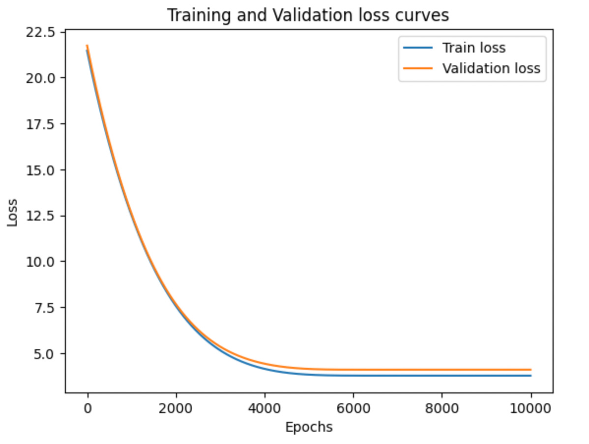
Looking at the train and validation loss curves we don’t see evidence of overfitting and from the training loop output we see that our train loss tends to converge around 3.772 and our validation loss converges around 4.096.
When we look at the state dict for our simple model, we can see that the weight is 4.3867 and the bias is 3.0133 which is really pretty close to our true weight and bias of 4.341 and 3.0. Also, remember that the weight/coefficient and bias from our sklearn model generated the same values as our pytorch model (4.3867 and 3.0133).
model.state_dict()OrderedDict([('linear.weight', tensor([[4.3867]], device='cuda:0')),
('linear.bias', tensor([3.0133], device='cuda:0'))])If we look at the R2 and MSE scores for our PyTorch modes we see that we are getting the same scores as our sklearn model. Pretty cool!
y_preds = predict(model, X_test, device=device)
r2 = R2Score().to(device)
r2.update(y_preds, y_test.to(device))
print(f"R2: {r2.compute()}")

mse = MeanSquaredError().to(device)
mse.update(y_preds, y_test.to(device))
print(f"MSE: {mse.compute()}")
R2: 0.7943850755691528
MSE: 4.218369960784912Getting Spicy with Simple Non-Linear Data
Okay, so that was pretty fun, but what happens when our data isn’t linear? What will the R2 and MSE scores look like in our simple sklearn model, and can we build a more complex PyTorch model to handle the non-linear data? (hint: yes, yes we can)
To create a non-linear dataset, let’s take our original data and send it through the sine function to make it more sinusoidal.
X, y, coef = make_regression(n_samples=1200, n_features=1, bias=bias, noise=2, random_state=42, shuffle=True, coef=True)

y_new = np.sin(2*X)+ np.random.normal(scale=0.1,size=len(X)).reshape(len(X),1)
X_new = X

X_train, X_val, y_train, y_val = train_test_split(X_new[:1000], y_new[:1000], test_size=0.20, random_state=42, shuffle=True)

X_train = torch.tensor(X_train, dtype=torch.float)
X_val = torch.tensor(X_val, dtype=torch.float)
y_train = torch.tensor(y_train, dtype=torch.float)# .unsqueeze(dim=1)
y_val = torch.tensor(y_val, dtype=torch.float)# .unsqueeze(dim=1)

X_test, y_test = X_new[1000:], y_new[1000:]
X_test = torch.tensor(X_test, dtype=torch.float)
y_test = torch.tensor(y_test, dtype=torch.float)# .unsqueeze(dim=1)

plt.scatter(X_new, y_new, alpha=0.5)
plt.xlabel("X")
plt.ylabel("y")
plt.tight_layout()
plt.show()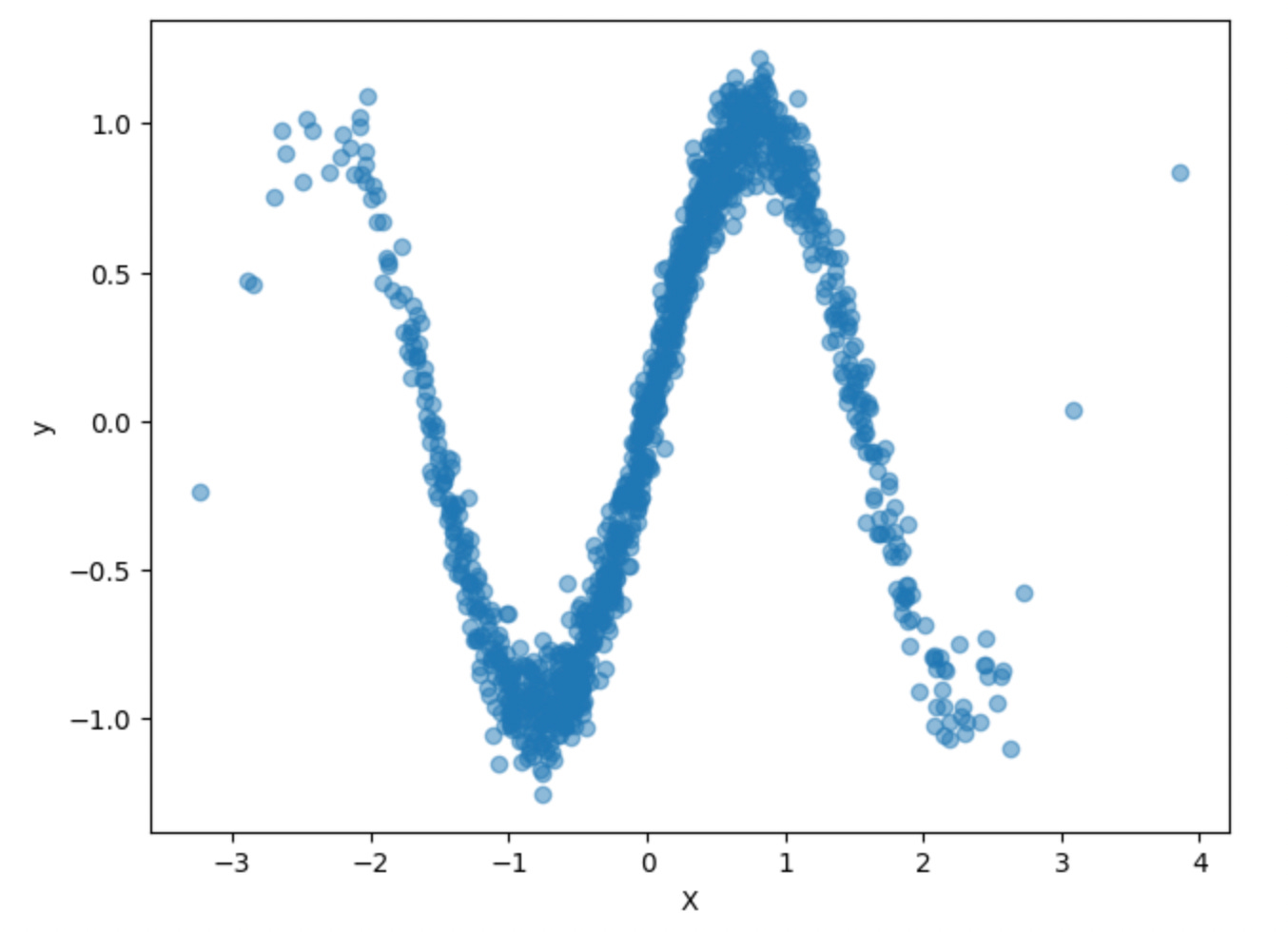
Next, let see how sklearn’s LinearRegression performs on this dataset.
np.random.seed(42)

lr = LinearRegression()
lr.fit(X_train, y_train)
y_pred =  lr.predict(X_test)
r2_score(y_test, y_pred)
print(f"coef: {lr.coef_[0][0]}")
print(f"bias: {lr.intercept_[0]}")
print(f"R2: {r2_score(y_test, y_pred)}")
print(f"MSE: {mean_squared_error(y_test, y_pred)}")
coef: 0.2958149015903473
bias: 0.0005384758114814758
R2: 0.07936591219376243
MSE: 0.4692360758781433As we can see, this simple model explains roughly 8% of the variation in the data. Not great compared to our simple dataset where the model was roughly 79%.
When we plot the best-fit line to the data, it’s obvious that it doesn’t fit very well.
coef = lr.coef_[0][0]
bias = lr.intercept_[0]
coef_str = str(np.round(lr.coef_[0][0], 3))
bias_str = str(np.round(lr.intercept_[0], 3))
plt.scatter(X_new, y_new, alpha=0.5)
plt.plot(X, X*coef+bias, 'r-', alpha=0.4)
plt.xlabel("X")
plt.ylabel("y")
plt.text(1.5, 1, f"y={coef_str}X+{bias_str}")
plt.tight_layout()
plt.show()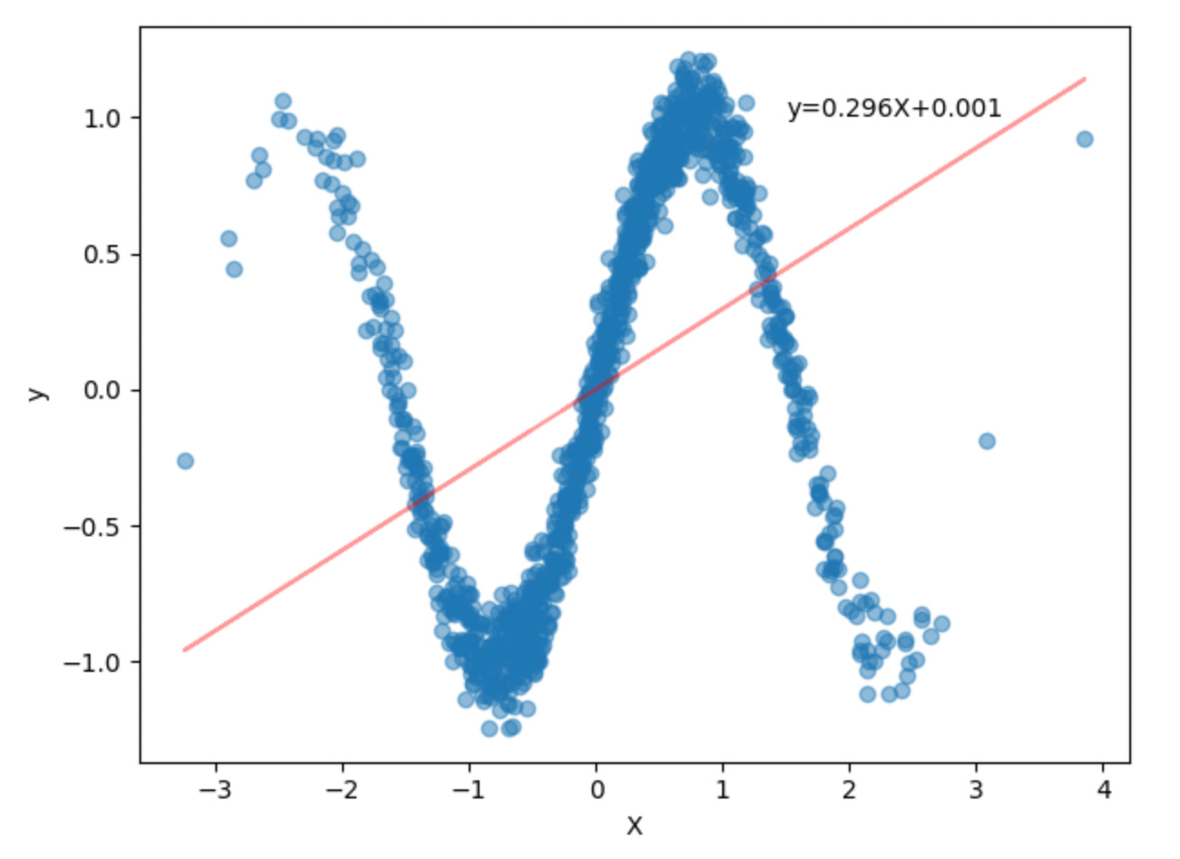
To help us with this problem, we need to develop a model that can handle non-linear data. In this model, we will use the ReLU (Rectified Linear Unit) activation function as it introduces non-linearity into the output of a node in a neural network.
ReLU(x)= max(0,x)The non-linearity of the ReLU activation function allows the network to capture complex patterns and interactions in the data that linear models cannot.
In classification problems, it helps to create complex decision boundaries, while for regression tasks, it enables the network to approximate non-linear functions when modeling real-world data.
Below is the model we will use for our sinusoidal data set. In this model, we will have one input layer, two hidden layers, and a final output layer. We will pass the output into the ReLU activation function for each of the first three layers while.
class non_linear_model(nn.Module):
    def __init__(self, in_features=1, hidden_units=8, out_features=1):
        super().__init__()
        self.linear_layer_stack = nn.Sequential(
            #1
            nn.Linear(in_features=in_features, out_features=hidden_units),
            nn.ReLU(),
            #2
            nn.Linear(in_features=hidden_units, out_features=hidden_units),
            nn.ReLU(),
            #3
            nn.Linear(in_features=hidden_units, out_features=hidden_units),
            nn.ReLU(),
            # final
            nn.Linear(in_features=hidden_units, out_features=out_features),
        )
    def forward(self, x):
        return self.linear_layer_stack(x)
As with the simple linear model, to train the new non-linear model, we can simply call an instance of our non_linear_model() class and then pass it into the training loop along with the training and validation data. Once our training loop has completed, we plot out the train and validation curves.
torch.manual_seed(42)

model = non_linear_model()

train_loss_values, val_loss_values, epoch_count = training_loop(model,
                                                                X_train,
                                                                y_train,
                                                                X_val,
                                                                y_val,
                                                                epochs = 10000, seed=42, device=device)

plot_losses(train_loss_values, val_loss_values, epoch_count)
Epoch: 0 | Train Loss: 0.5030714273452759 | Validation Loss: 0.5128653645515442
Epoch: 1000 | Train Loss: 0.01010216772556305 | Validation Loss: 0.02050055004656315
Epoch: 2000 | Train Loss: 0.009800932370126247 | Validation Loss: 0.01999005302786827
Epoch: 3000 | Train Loss: 0.009652948006987572 | Validation Loss: 0.019086314365267754
Epoch: 4000 | Train Loss: 0.009528052993118763 | Validation Loss: 0.018076639622449875
Epoch: 5000 | Train Loss: 0.009423813782632351 | Validation Loss: 0.0172061026096344
Epoch: 6000 | Train Loss: 0.009330359287559986 | Validation Loss: 0.0162790697067976
Epoch: 7000 | Train Loss: 0.00926120299845934 | Validation Loss: 0.015430329367518425
Epoch: 8000 | Train Loss: 0.00921510811895132 | Validation Loss: 0.014866281300783157
Epoch: 9000 | Train Loss: 0.009186663664877415 | Validation Loss: 0.014394217170774937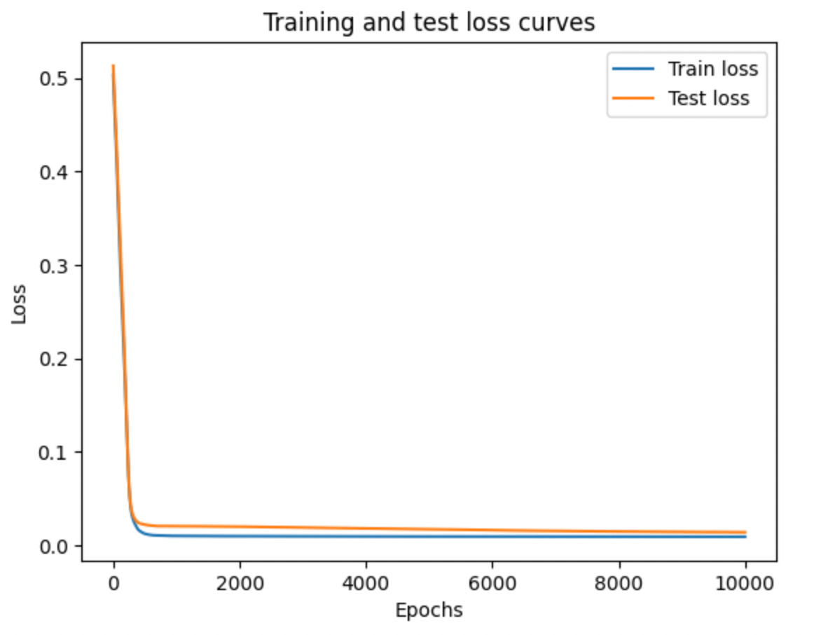
Even running 10,000 epochs it seems our train and validation losses are continuing to decrease, albeit minimally. Taking a look at the R2 and MSE scores, we see that this new model explains roughly 98% of the variation in the data and our MSE is 0.012 which is great compared to our simple linear model.
y_preds = predict(model, X_test, device=device)
r2 = R2Score().to(device)
r2.update(y_preds, y_test.to(device))
print(f"R2: {r2.compute()}")

mse = MeanSquaredError().to(device)
mse.update(y_preds, y_test.to(device))
print(f"MSE: {mse.compute()}")
R2: 0.9768771529197693
MSE: 0.011785447597503662Out of curiosity we can look at the state dictionary for our model. Note that we no longer have a nice single weight/coefficient and bias/intercept with this more complex model.
model.state_dict()OrderedDict([('linear_layer_stack.0.weight',
tensor([[ 0.6768],
[ 1.2384],
[ 0.3777],
[ 1.1293],
[-0.3951],
[ 0.3451],
[-0.7082],
[ 0.9536]], device='cuda:0')),
('linear_layer_stack.0.bias',
tensor([ 1.4948, -1.1457, 1.4129, 0.4750, 0.7310, 0.4192, 0.6129, 0.0232],
device='cuda:0')),
('linear_layer_stack.2.weight',
tensor([[ 0.4271, 0.2132, -0.2128, 0.3714, -0.3537, 0.2050, -0.6378, 0.6161],
[-1.2124, -0.1630, 0.4892, -0.2126, 0.2193, 0.6140, 0.4916, -0.3003],
[ 0.0668, -0.3504, 0.3612, 0.0698, 0.1426, 0.1445, -0.3280, -0.3548],
[-0.2114, -0.4891, 0.4720, 0.4142, 0.3180, -0.0891, -0.0574, -0.0275],
[ 0.3126, -0.7116, -0.1272, -0.0980, -0.1410, 0.3732, -0.2229, -0.0448],
[ 0.5330, -0.0062, 0.0915, -0.5669, 0.0520, -0.5426, 0.3431, -0.4357],
[ 0.3199, -1.2057, 0.4745, -0.5479, 0.0190, -0.4350, 0.5202, -0.3022],
[ 0.3298, -0.3021, -0.3507, -0.2870, -0.2378, 0.1328, 0.1266, 0.2834]],
device='cuda:0')),
('linear_layer_stack.2.bias',
tensor([-0.1237, -0.3341, 0.6843, 0.2014, 0.3867, -0.2428, 0.4570, -0.2851],
device='cuda:0')),
('linear_layer_stack.4.weight',
tensor([[-0.1935, 0.1078, 0.0590, -0.1058, 0.1951, 0.2247, -0.2721, -0.1888],
[ 0.6514, -0.1193, -0.9506, -1.1978, -0.3797, 0.0883, -0.0467, -0.2566],
[-0.1532, -0.7266, 0.0049, -0.1939, 0.4226, 0.1650, 0.4821, 0.0668],
[ 0.0519, -0.3298, -0.2707, -0.1709, 0.0553, -0.3111, -0.1523, -0.2117],
[-0.1635, -0.1316, 0.1905, 0.0138, 0.0296, -0.1401, -0.3034, -0.2791],
[ 0.4255, -0.7782, 0.1335, -0.2771, -0.9717, 0.5068, 0.1821, -0.1436],
[-0.4813, -1.1457, 0.1297, -0.2832, -0.1043, 0.1330, 0.5264, -0.2595],
[-0.3258, 0.6291, 0.3938, 0.6025, 0.4206, -0.6692, -0.0332, -0.1439]],
device='cuda:0')),
('linear_layer_stack.4.bias',
tensor([-0.0545, -1.0524, 0.2333, -0.3137, 0.4232, 0.2744, 0.3879, 0.1250],
device='cuda:0')),
('linear_layer_stack.6.weight',
tensor([[ 0.3175, 1.1241, -0.1428, -0.2684, 0.4165, -0.5978, -0.5955, 0.6898]],
device='cuda:0')),
('linear_layer_stack.6.bias', tensor([0.0679], device='cuda:0'))])Conclusion
In this post, we saw how to build a simple learn regression model using PyTorch then compared the results with the sklearn linear regression implementation. We then looked at the limitations of trying to fit the sklearn implementation to non-linear data and showed how we can build a PyTorch model using the ReLU activation function to help us approximate non-linear functions in our neural network to help capture complex patterns and interactions in the data.