Predicting IoT Adversarial Network Behaviors
Neural Networks versus Bagging and Boosting methods


In my previous roles at Hitachi, I was fortunate to work with some very smart folks in the Industrial IoT (IIoT) space. This experience sparked a serious appreciation of what it takes to manage a production IIoT environment. In working with these teams, I was able to work as both a technical product manager, helping the more senior team members research the product landscape as well as working with development teams to develop test code for IIoT platforms. One thing that always stuck with me was how much data and the types of data these systems generated. At the time, I was just beginning my journey into data science and never got the opportunity to wrestle with the data. Now that I'm finishing up my master's, I wanted to go back and play with some of that data, but unfortunately, there aren't many public IoT data sets available. After doing a bit of digging, the UCI Machine Learning Repository had an interesting dataset from Rohini Nagapadma, et. al. that accompanied their paper, "Quantized autoencoder (QAE) intrusion detection system for anomaly detection in resource-constrained IoT devices using RT-IoT2022 dataset".
Rohini Nagapadma, et. al. describe the dataset this way:
The RT-IoT2022, a proprietary dataset derived from a real-time IoT infrastructure, is introduced as a comprehensive resource integrating a diverse range of IoT devices and sophisticated network attack methodologies. This dataset encompasses both normal and adversarial network behaviours, providing a general representation of real-world scenarios. Incorporating data from IoT devices such as ThingSpeak-LED, Wipro-Bulb, and MQTT-Temp, as well as simulated attack scenarios involving Brute-Force SSH attacks, DDoS attacks using Hping and Slowloris, and Nmap patterns, RT-IoT2022 offers a detailed perspective on the complex nature of network traffic. The bidirectional attributes of network traffic are meticulously captured using the Zeek network monitoring tool and the Flowmeter plugin. Researchers can leverage the RT-IoT2022 dataset to advance the capabilities of Intrusion Detection Systems (IDS), fostering the development of robust and adaptive security solutions for real-time IoT networks.
For this post, I simply want to see if we can build a classification model to detect the differences between normal and adversarial IoT network behaviors. After building the model, we will compare the results with those of more "traditional" bagging and boosting methods.
The Data
Before building and actually training the models, let's take a look at what the data looks like.
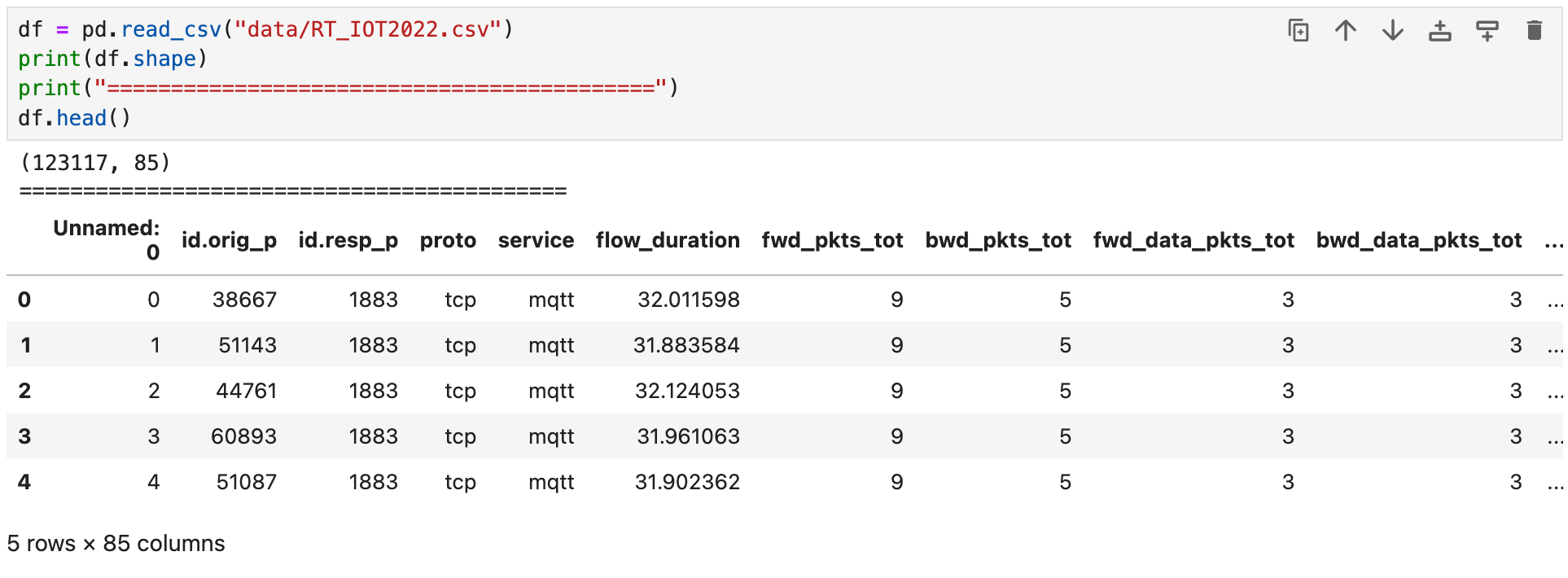
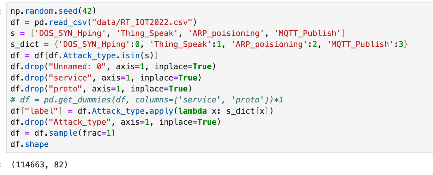
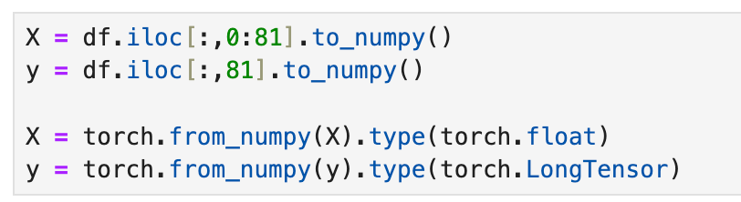
When we load the data, we get 123117 data points with 85 features. Looking at the first few rows of the data, we can already see that we'll need to drop the "Unnamed: 0" column.
When we plot the label distribution, it's clear that the dataset is heavily skewed toward the "DOS_SYN_Hping" data points. This means the dataset is imbalanced, and we will have to deal with that when we train our models.
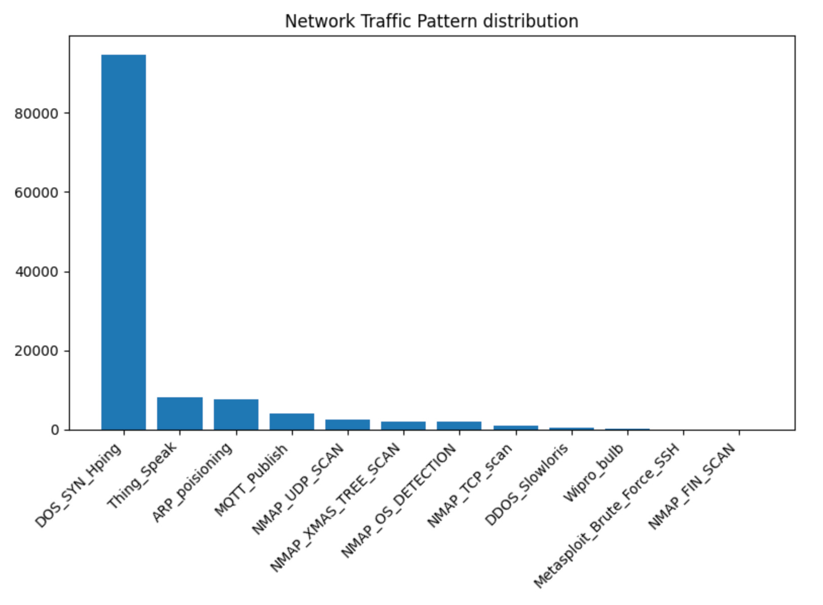
For this exercise, let's use the top 4 labels:
DOS_SYN_Hping,
Thing_Speak,
ARP_poisioning
MQTT_Publish.
Of these 4 IoT traffic patterns, DOS_SYN_Hping and ARP_poisioning are network attack patterns, while Thing_Speak and MQTT_Publish are "normal" IoT traffic patterns. By selecting these traffic patterns, we still have 114663 data points out of the original 123117. In addition to only selecting the top 4 traffic patterns, we will drop the "service" and "proto" features.
Sample Weights
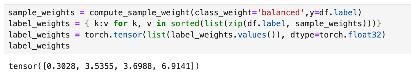
Once we've cleaned up the data, we need to generate the sample weights for our dataset, which will help us deal with the imbalances in our data.
How do these sample weights help us deal with imbalances in our data? In our PyTorch classification model, we will use CrossEntropyLoss as our loss function. If we look at the CrossEntropyLoss documentation, there is an option to pass the function a weight tensor that serves as "a manual rescaling weight given to each class." We use the weights calculated below with our cross-entropy loss function.
To calculate the sample weights, we will use the scikit-learn function compute_sample_weight. This function estimates the sample weights by class for our unbalanced dataset. We will use this function for the PyTorch and XGBoost models we will build; RandomForest typically can handle imbalanced datasets.
PyTorch
As with previous posts, we’ll use PyTorch to build our model. Since we are trying to distinguish between adversarial network behaviors, we will need to build a multiclass classifier that can detect valid traffic, such as MQTT and Thing Speak traffic, and malicious network traffic, such as denial of service and ARP poisoning attacks.
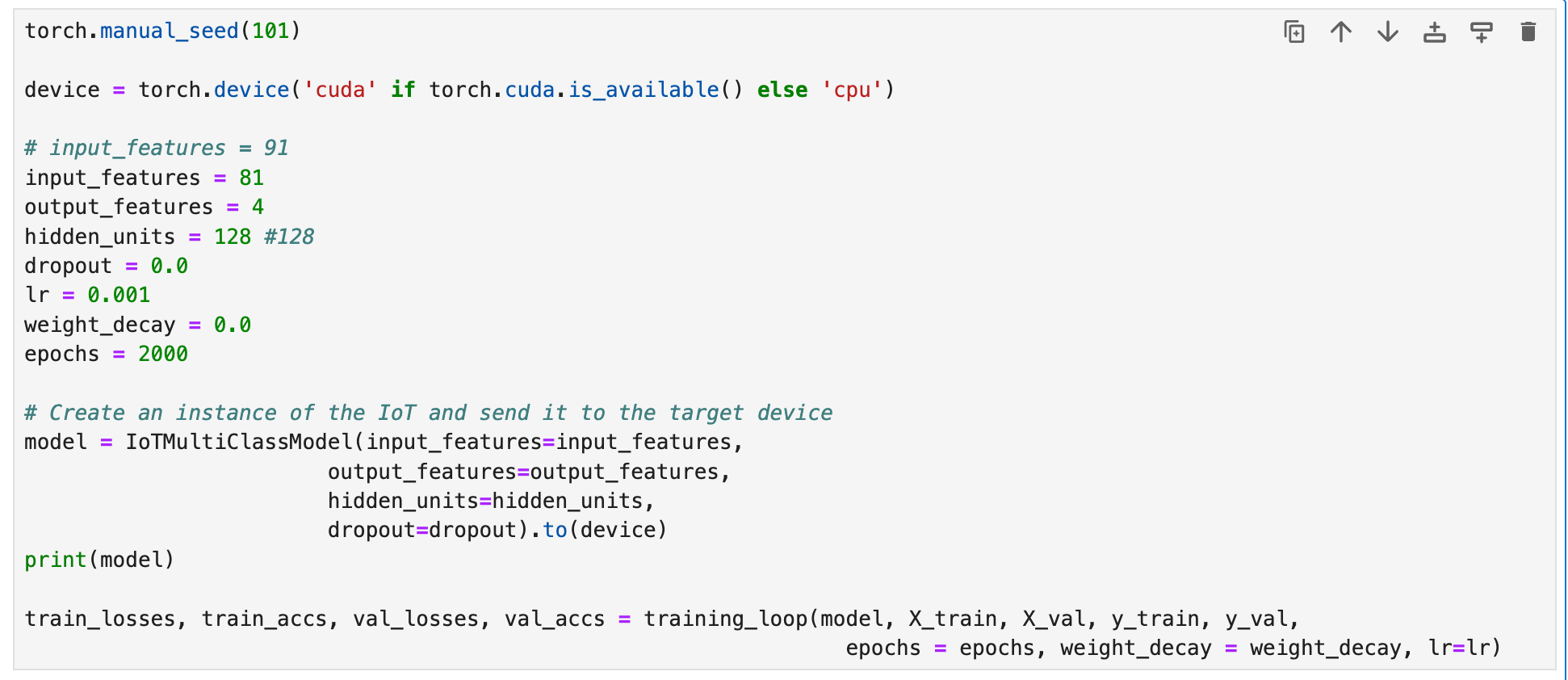
To help us with this problem, we will construct a model that takes 81 input features, 4 outputs, and 10 hidden layers with 128 neurons per layer. The model that I created is shown below. The 81 input features correspond to the 81 features from our data (minus "service" and "proto"). The 4 output features correspond to our 4 labels: DOS_SYN_Hping, Thing_Speak, ARP_poisioning and MQTT_Publish.
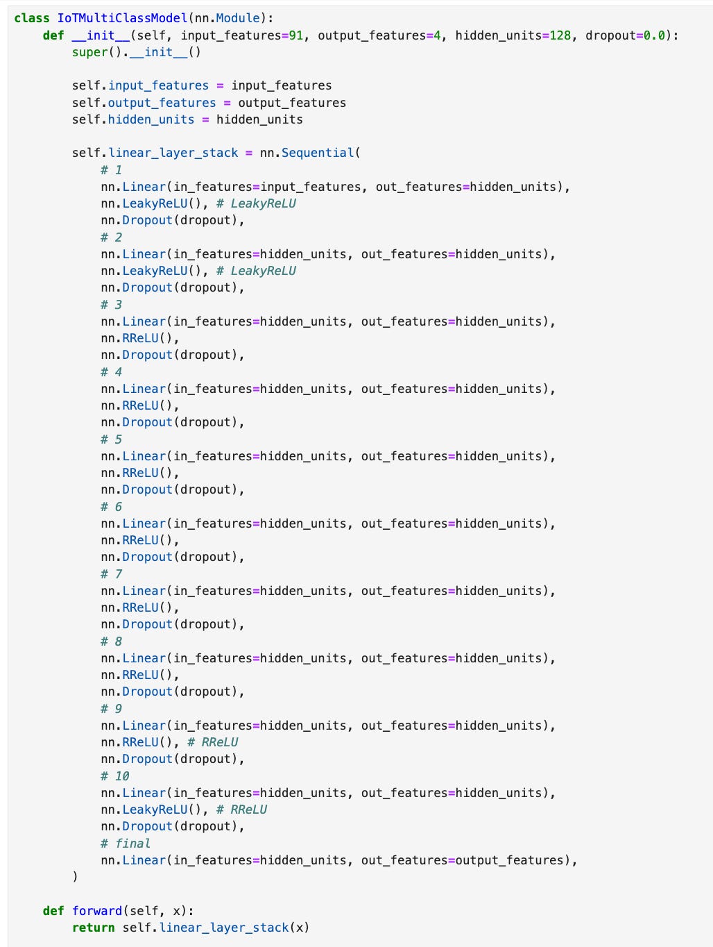
Link to GitHub Gist PyTorch Model
The training loop used with this model is shown below. It takes the training and validation data and places it on the specified device (cpu or gpu). We will use the torchmetrics accuracy function to calculate the accuracy at each epoch. CrossEntropyLoss is used because this is a multiclass classification problem and we will use the Adam optimizer.
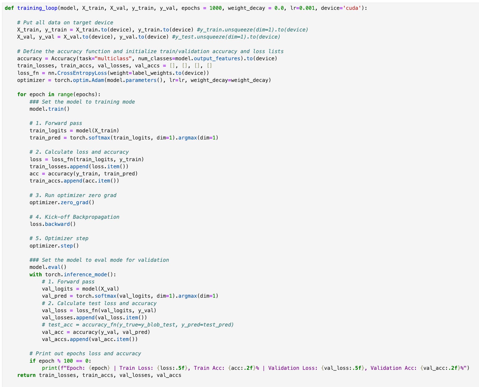
Link to GitHub Gist Training Loop
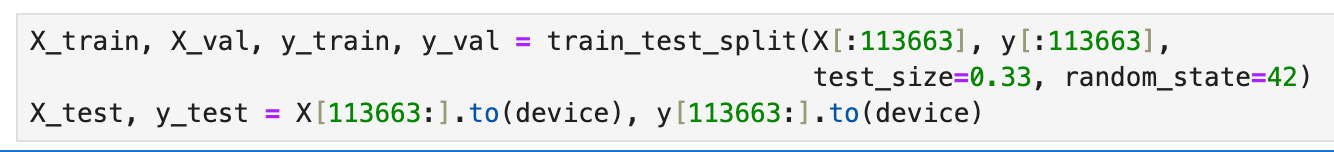
Before training the model, we need to do a bit of setup by converting the data to pytorch tensors, then split the data into train, validation, and test sets.
After splitting the data, we can start training the model. Even though we included dropout layers in the model, we will set the dropout probability and weight decay to zero. Both dropout (aka dropout regularization) and weight decay (aka L2 regularization) are regularization methods that help with overfitting. If our model is overfitting the data, we can try to tweak the dropout and weight decay parameters.
Example output from the training loop. Printing the model object, will display the model architecture.
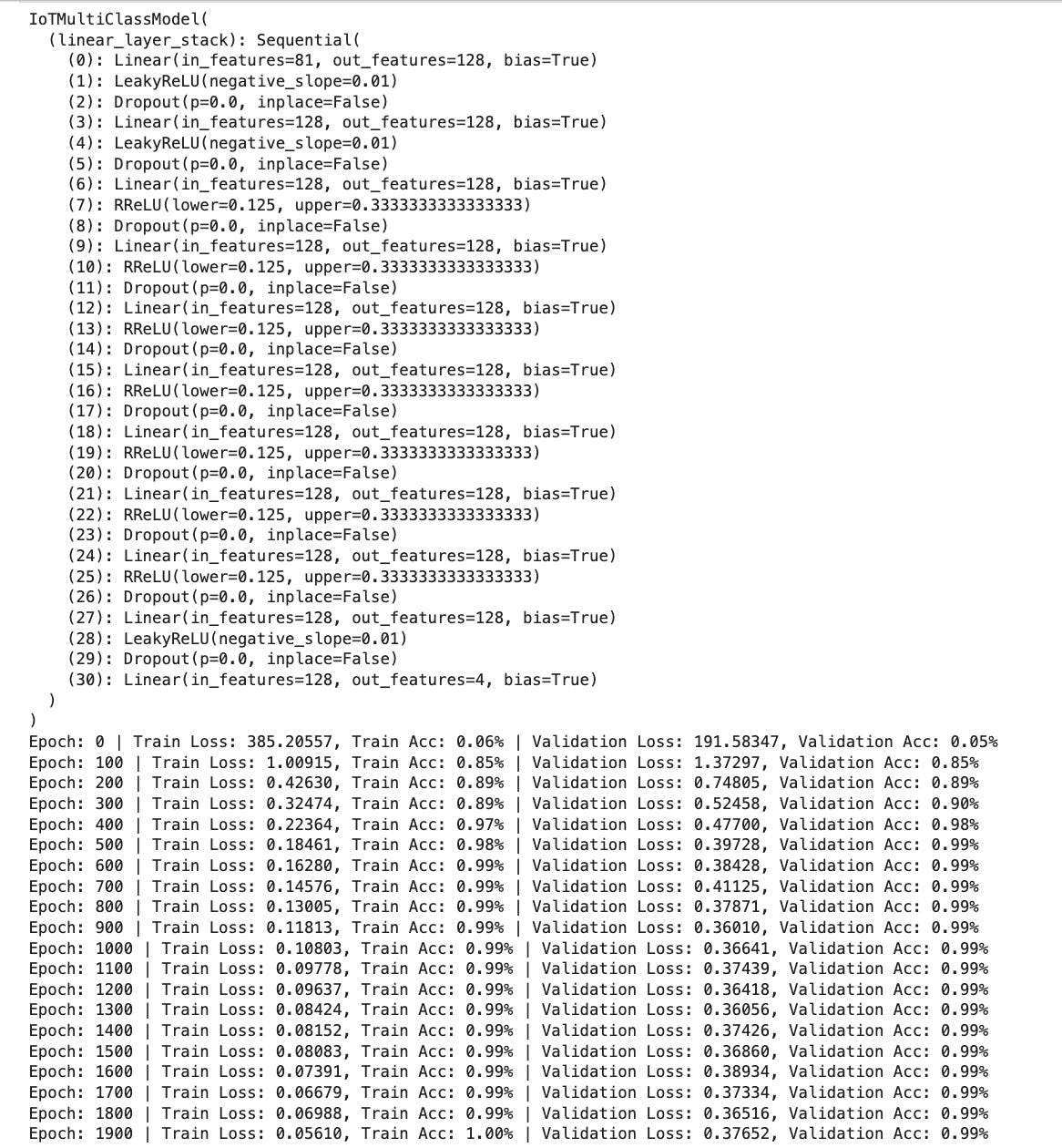
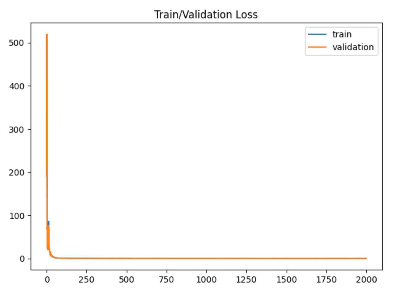
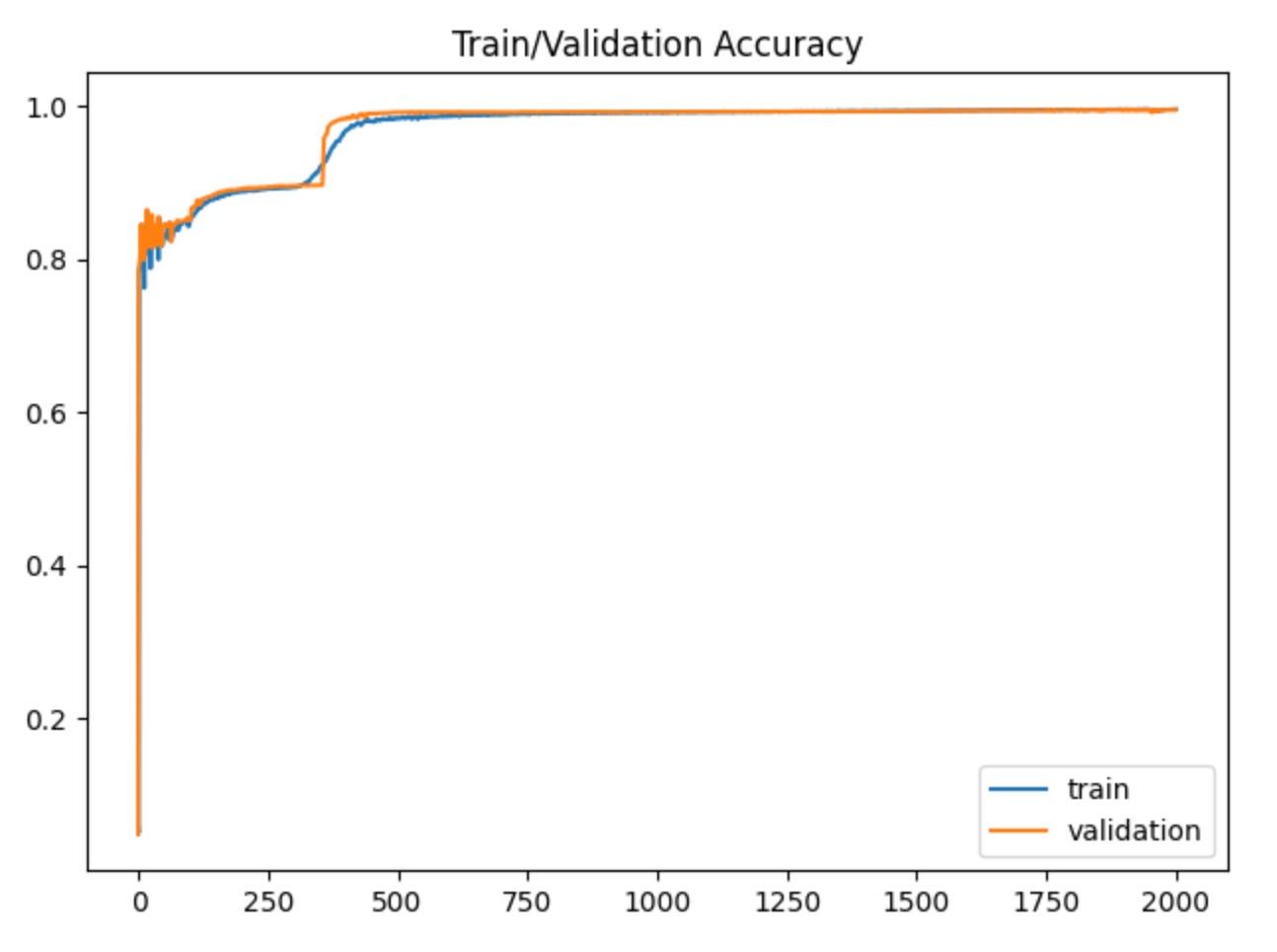
Plotting out our losses and accuracy, we can see that our model isn’t overfitting the data, which is good.
Now that the model has been trained, we can evaluate on the test dataset.
Because our dataset was imbalanced, we used the sample weights and passed them into the loss function to help deal with those imbalances. Additionally, because accuracy metrics can be misleading when dealing with imbalanced data, we will also look at precision, recall and f1-scores.

Looking at the accuracy for the test data, we get 99.9%, and the confusion matrix backs this up, showing that the model only misclassified one data point. When we run the classification report command, the precision, recal and f1-scores back up our accuracy score. All-in-all, this model does really well on the data, but can we get the same or better results with a boosting (XGboost) or bagging (Random Forest) approach? Let’s see!
XGBoost
Before building our XGBoost model, let’s combine the training and validation data so that we simply have train and test datasets.
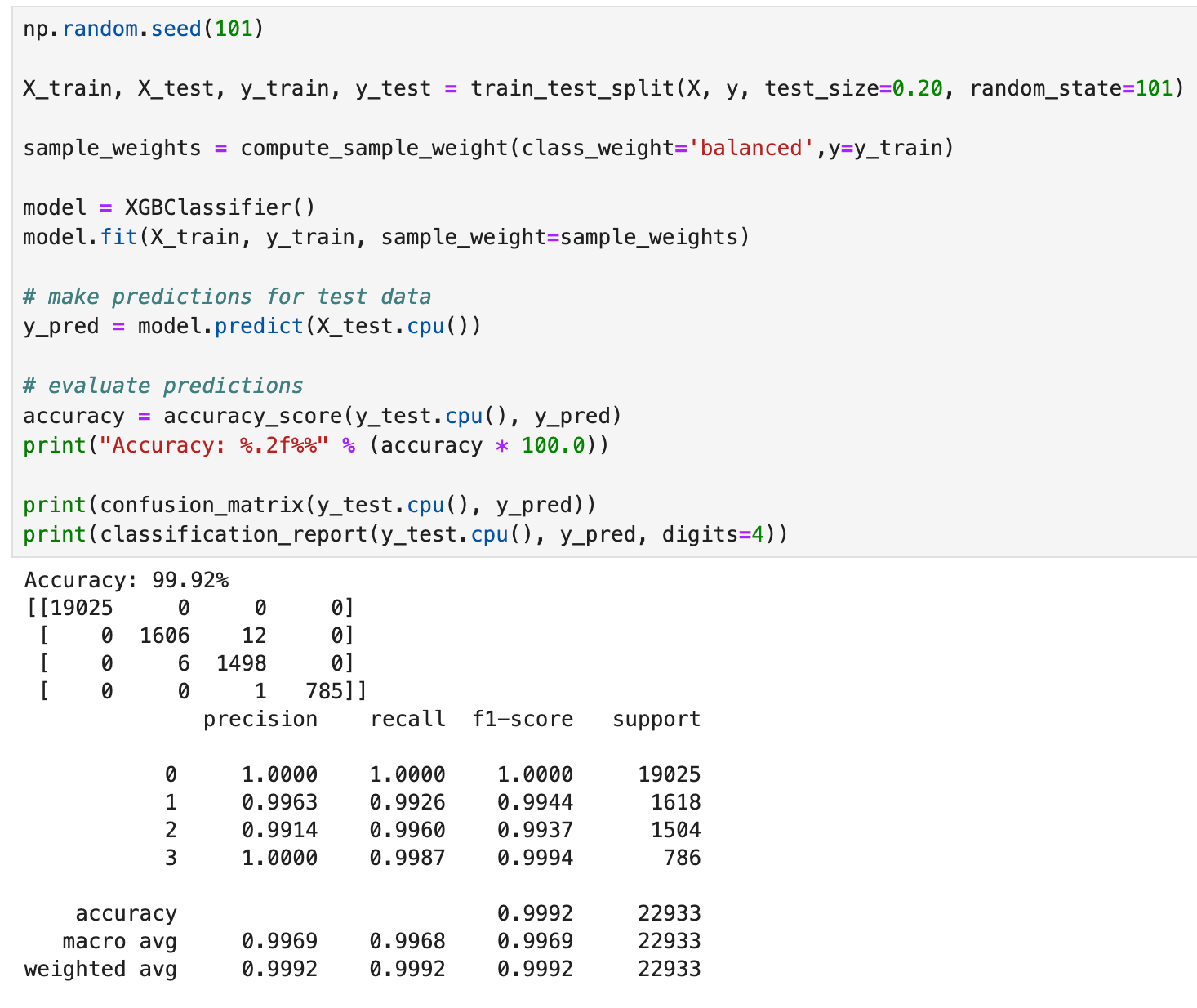
Next, we can load the XGBClassifier and fit the training data with the sample weights. XGBoost has different options to help deal with imbalanced classes. For our case, we will use the sample_weight parameter in the fit method. The sample_weight parameter allows us to specify a different weight for each training sample, whereas the scale_pos_weight parameter in the XGBClassifer method lets us provide a weight for an entire class in the samples.
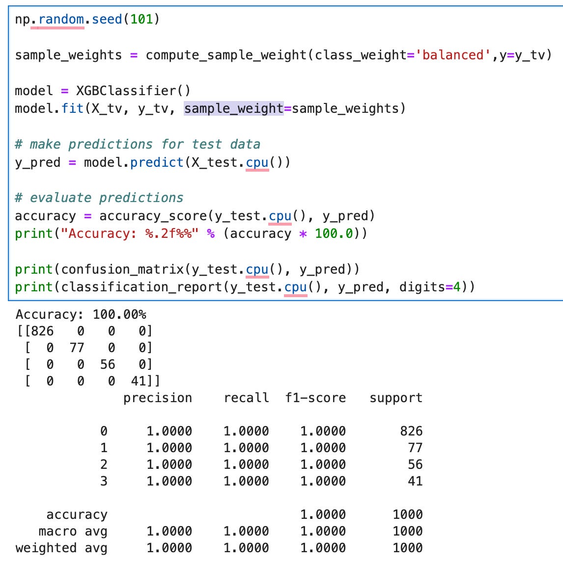
Checking the accuracy and confusion matrix for the test predictions shows that we were able to classify all the test samples correctly; this is pretty amazing for an “out-of-the-box” model! Next let’s see if we do the same thing with good old Random Forest.
Random Forest
Okay, so we’ve seen how our pytorch and XGBoost classifiers perform, but what about good ol’ Random Forest?
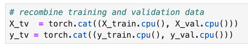
Once again, we will combine the train and validation data so that we simply have train and test datasets.
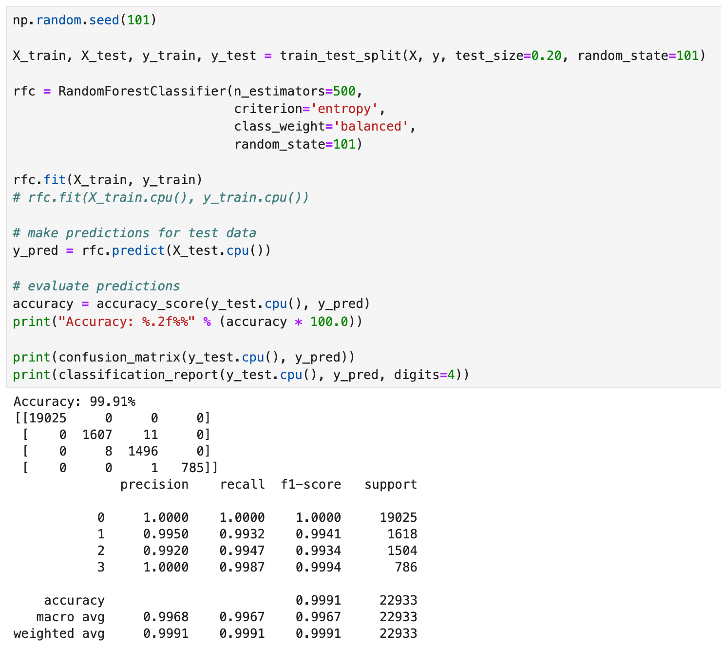
Next let’s go ahead and pass in the training data into a RandomForestClassifier and check the performance of our model. Note when we used our pytorch model and the XGBoost model, we had to specific the class weights. The sklearn implementation of the RandomForestClassifier will take care of that for you when you specify the class_weight parameter as “balanced”.
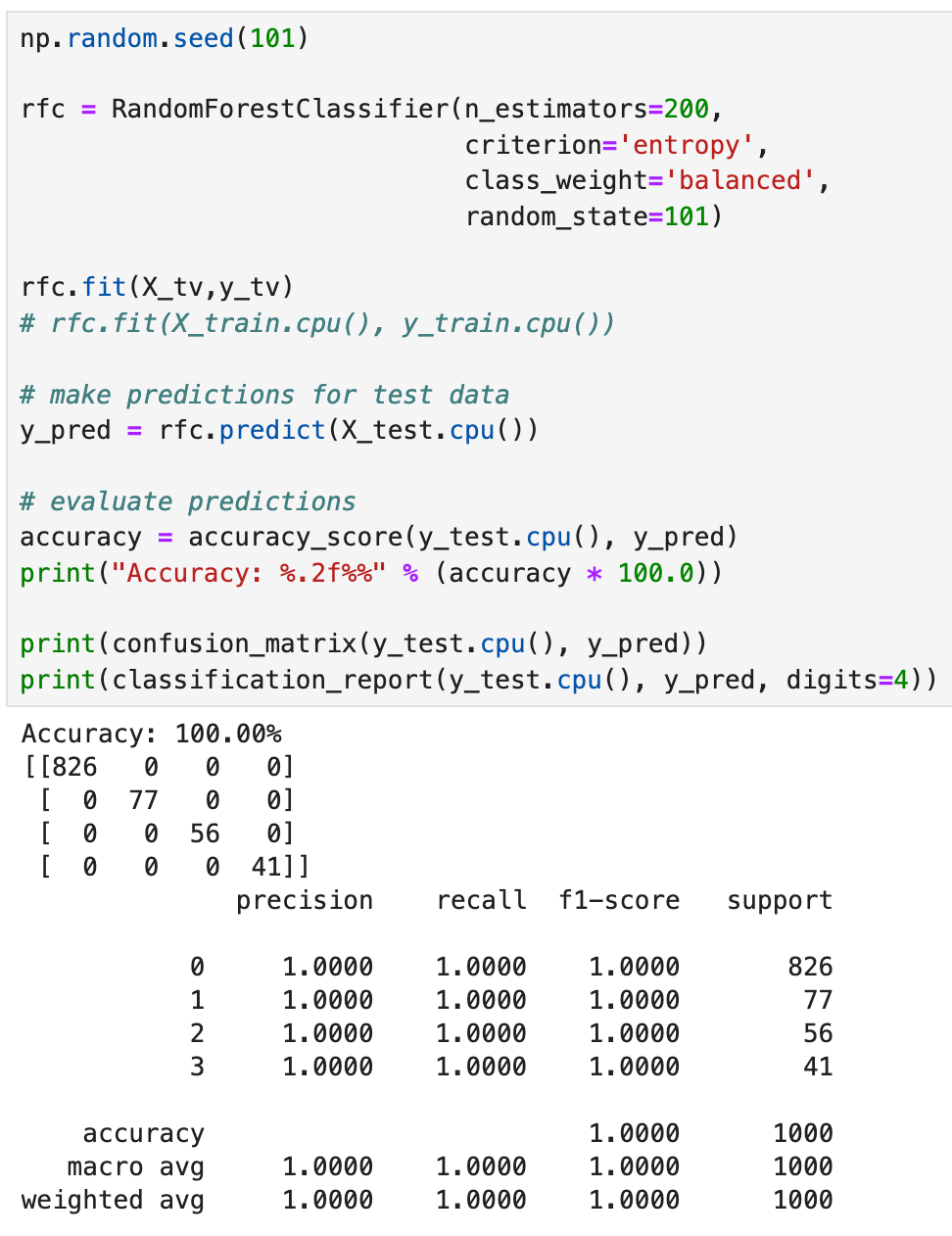
Like the XGBClassifier, we get an accuracy of 100%, with the confusion matrix showing no misclassifications. Again, like the XGBClassifier, our precision, recal and f1-scores were 100%. This is fantastic!
One thing to note is that the RandomForest algorithm seemed to take a bit longer than the XGBClassifier. In terms of training time, the XGBClassifier was the fastest with the pytorch model taking the longest.
Conclusion
When we looked at boosting and bagging methods, we were able to classify correctly all the data points where our pytorch model was not.
Some folks might take issue with the fact that I recombined the training and validation sets, leaving a smaller test set. In subsequent tests where we re-split the data into an 80/20 split, we get similar results to our pytorch model. This is something to keep in the back of our minds when comparing the performance of different models; how you split the data and any random effects associated with that could affect your results.
Ultimately, the bagging and boosting methods tend to perform slightly better when we consider the precision, recall, and F1 scores of our various models.