
Exploring Expectation Maximization
Latent Variables, Expectation Maximization and Gaussian Mixture Models

In my last post, I tried to tackle the concept of maximum likelihood estimation (MLE). In this post, I want to grapple with the idea of expectation maximization but before doing so I want talk about the idea of latent variables and why they drive the need for expectation maximization.
Latent Variables
In statistics, latent variables are variables that are not directly observed but are inferred from other variables that are observed (measured). They are often used to represent abstract concepts or constructs that cannot be measured directly but influence the observed data. Wikipedia states that latent variables “are variables that can only be inferred indirectly through a mathematical model from other observable variables that can be directly observed or measured.”
To help wrap our minds around this concept, consider a dataset generated from multiple Gaussian distributions (clusters), but you don't know which data point belongs to which Gaussian. The hidden variables are the cluster assignments.
As a set of more concrete examples, latent variables can be seen:
In natural language processing models like Latent Dirichlet Allocation (LDA), the actual topic is a latent variable inferred from the words in a document.
In recommender systems, latent preferences are inferred based on user behavior such as ratings, clicks, or purchase history
In customer satisfaction surveys, satisfaction is inferred from responses to specific questions about a product or service.
In economics, market sentiment is a latent variable representing investor behavior or expectations, which can be inferred from stock prices, trading volumes, or volatility.
How does this idea of latent variables impact maximum likelihood estimation and how does it lead us to the idea of expectation maximization?
From my previous post, we learned that maximum likelihood estimation (MLE) is a method for estimating the parameters of a statistical model given a dataset and that it involves finding the values of the model parameters that maximize the likelihood function of the observed data given the model. According to Jason Brownlee, it is a framework for “estimating the probability distribution for a sample of observations from a problem domain”. Essentially, it “is an approach to density estimation for a dataset by searching across probability distributions and their parameters”.
Coming back to the concept of latent variables, we find that when our data is “complete” and does not contain any latent or missing variables, MLE is a tractable problem than can be solved with analytical methods such as taking the derivative of the likelihood (or log-likelihood) function with respect to the various parameters and solving.
When we have latent or missing data, MLE becomes more difficult and in many cases the problem becomes intractable which means we need some kind of iterative approach to finding the parameters of our model.
EM Algorithm
Expectation Maximization (EM) is an iterative algorithm used for finding the maximum likelihood estimates of parameters in statistical models, especially when the data has missing or hidden variables. It becomes important in problems where direct computation of the likelihood function is difficult, such as in clustering (e.g., Gaussian Mixture Models), latent variable models, and incomplete data scenarios.
Larry Wasserman describes the general idea of expectation maximization this way:
The idea is to iterate between taking an expectation then maximizing. Suppose we have data 𝑌 whose density 𝑓(𝑦;𝜃) leads to a log-likelihood that is hard to maximize. But suppose we can find another random variable 𝑍 such that 𝑓(𝑦;𝜃)=∫𝑓(𝑦,𝑧;𝜃)𝑑𝑧 and such that the likelihood based on 𝑓(𝑦,𝑧;𝜃) is easy to maximize. In other words, the model of interest is the marginal of a model with a simpler likelihood. In this case, we call Y the observed data and Z the hidden (or latent or missing) data. If we could just "fill in" the missing data, we would have an easy problem. Conceptually, the EM algorithm works by filling in the missing data, maximizing the log-likelihood, and iterating.
EM exploits the fact that if the data were fully observed, then the MLE would be easy to compute. In particular, EM alternates between inferring the missing values given the parameters (E step), and then optimizing the parameters given the “filled in” data (M step).
The general form of the EM Algorithm is described below (ref: Bishop):
Given a joint distribution p(Y, Z|θ) which generates a set of observed variables Y and a set of unobserved, latent variables Z, and vector of unknown parameters θ, the goal is to maximize the likelihood function p(Y|θ) with respect to θ.
Choose an initial setting for the parameters θt-1
E-step: Evaluate p(Z|Y,θt-1)
M-step: Evaluate θt given by:
where
Check for convergence of the parameter values. If convergence is not met, then:
and return to the E-Step.
Gaussian Mixture Model
Utilizing this general form, we can apply it to Gaussian mixtures. A Gaussian Mixture Model is a probabilistic model used to represent data that is generated from a mixture of several Gaussian distributions.
Bishop, again with the general form of EM for Gaussian Mixtures:
Given a Gaussian mixture model, the goal is to maximize the likelihood function with respect to the parameters μk, Σk, and πk.
Initialize the means μk, covariances Σk and mixing coefficients πk, and evaluate the initial value of the log likelihood.
E-step. Evaluate the responsibilities using the current parameter values:
M-step. Re-estimate the parameters using the current responsibilities:
where
Evaluate the log likelihood
and check for convergence of either the parameters or the log likelihood. If
the convergence criterion is not satisfied return to step 2.
Gaussian Mixture Model Python Implementation
To implement a Gaussian Mixture Model (GMM) in python, we can start by importing the necessary libraries and then creating a dataset.
import numpy as np
from scipy.stats import norm
import matplotlib.pyplot as plt
To test out our GMM implementation, let’s create a dataset comprised of three different gaussian distributions with the means being centered at 0.0, 5.0 and 10. We set the standard deviations to 1.0, 1.24 and 1.5 respectively.
np.random.seed(101)

n_samples = 1000000
mu = [0.0, 5.0, 10]
var = [1.0, 1.25, 1.5]
d1 = np.random.normal(loc=mu[0], scale=var[0], size=n_samples)
d2 = np.random.normal(loc=mu[1], scale=var[1], size=n_samples)
d3 = np.random.normal(loc=mu[2], scale=var[2], size=n_samples)
X = np.concatenate((d1,d2,d3))
To view the mixture of our dataset, let’s plot it out. As we can see we have three different normal distributions. If we try to fit a single normal distribution to this dataset, it won’t fit it well, hence the need for a gaussian mixture model.
plt.hist(d1, bins=100, density=True, alpha=0.5)
plt.hist(d2, bins=100, density=True, alpha=0.5)
plt.hist(d3, bins=100, density=True, alpha=0.5)
plt.tight_layout()
plt.show()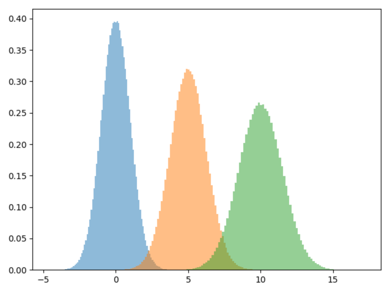
The following is a pure python implementation of a GMM. It takes the number of number of components or gaussian distributions, the max number of iterations and a random seed. The GMM class has two functions: the e-step function and the m-step function that both correspond to the E and M steps of the expectation maximization algorithm. Finally, there is a fit function to fit the model to the data.
class GMM:
    def __init__(self, n_components=3, max_iter=100, seed=42):
        np.random.seed(seed)
        self.n_components = n_components
        self.max_iter = max_iter
        self.pi = np.ones((n_components)) / n_components
        self.means = np.random.choice(X, n_components)
        self.variances = np.random.random_sample(size=n_components)
        self.X = None
        self.weights = None


    def e_step(self):
        self.weights = np.zeros((self.n_components,len(self.X)))
        for i in range(self.n_components):
            self.weights[i,:] = norm(loc=self.means[i],scale=np.sqrt(self.variances[i])).pdf(self.X)
        return self.weights

    def m_step(self):
        g = []
        for j in range(self.n_components):
            num = self.weights[j] * self.pi[j]
            den = np.sum([self.weights[i] * self.pi[i] for i in range(self.n_components)], axis=0)
            g.append(num / den)

            self.means[j] = np.sum(g[j] * self.X) / (np.sum(g[j]))
            self.variances[j] = np.sum(g[j] * np.square(self.X - self.means[j])) / (np.sum(g[j]))

            self.pi[j] = np.mean(g[j])

        return self.variances, self.means, self.pi

    def fit(self, X):
        self.X = X
        for step in range(self.max_iter ):
            self.weights = self.e_step()
            self.variances, self.means, self.pi = self.m_step()
After calling the GMM class and fitting the model to the data we see that it comes pretty close to the true means of 0, 5 and 10 and the square root of the variances come very close to our true standard deviations.
gmm = GMM()
gmm.fit(X)
print(f"means: {gmm.means}")
print(f"variances: {np.sqrt(gmm.variances)}")
means: [ 9.99951736e+00 -1.03162860e-03 4.99957139e+00]
variances: [1.50325037 1.00134846 1.24989789]Plotting out the true distributions against the predicted distribution, shows that our model does a pretty good job of fitting to the data.
plt.hist(d1, bins=100, density=True, alpha=0.5)
plt.hist(d2, bins=100, density=True, alpha=0.5)
plt.hist(d3, bins=100, density=True, alpha=0.5)

x = np.linspace(X.min(), X.max(), 1000)
y = norm.pdf(x, gmm.means[0], np.sqrt(gmm.variances[0]))
plt.plot(x, y, "k--")

y = norm.pdf(x, gmm.means[1], np.sqrt(gmm.variances[1]))
plt.plot(x, y, "--")

y = norm.pdf(x, gmm.means[2], np.sqrt(gmm.variances[2]))
plt.plot(x, y, "g--")

plt.tight_layout()
plt.show()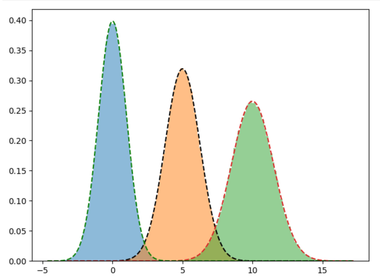
Comparison against the sklearn GMM implementation
So, how does our Gaussian Mixture Model implementation compare to scikit-learn’s implementation? To use the scikit-learn implementation, we call the GaussianMixture method, set the number of components to 3 then fit it to the data.
from sklearn.mixture import GaussianMixture

gm = GaussianMixture(n_components=3, random_state=42).fit(X.reshape(-1, 1))
We can see from the output that the means and covariances are very similar to what we found in the implementation above.
print(f"means: {[m[0] for m in gm.means_]}")
print(f"variances: {[v[0][0] for v in np.sqrt(gm.covariances_)]}")
means: [0.0069505769179209346, 5.042176062990392, 10.04512584482456]
variances: [1.0094546387836933, 1.2647646281341405, 1.4670591398449797]Again, when we plot the learned means and covariances from the scikit-learn implementation we get a very similar view and our pure python implementation.
plt.hist(d1, bins=100, density=True, alpha=0.5)
plt.hist(d2, bins=100, density=True, alpha=0.5)
plt.hist(d3, bins=100, density=True, alpha=0.5)

x = np.linspace(X.min(), X.max(), 1000)
y = norm.pdf(x, gm.means_[0][0], np.sqrt(gm.covariances_[0][0][0]))
plt.plot(x, y, "k--")

y = norm.pdf(x, gm.means_[1][0], np.sqrt(gm.covariances_[1][0][0]))
plt.plot(x, y, "--")

y = norm.pdf(x, gm.means_[2][0], np.sqrt(gm.covariances_[2][0][0]))
plt.plot(x, y, "g--")

plt.tight_layout()
plt.show()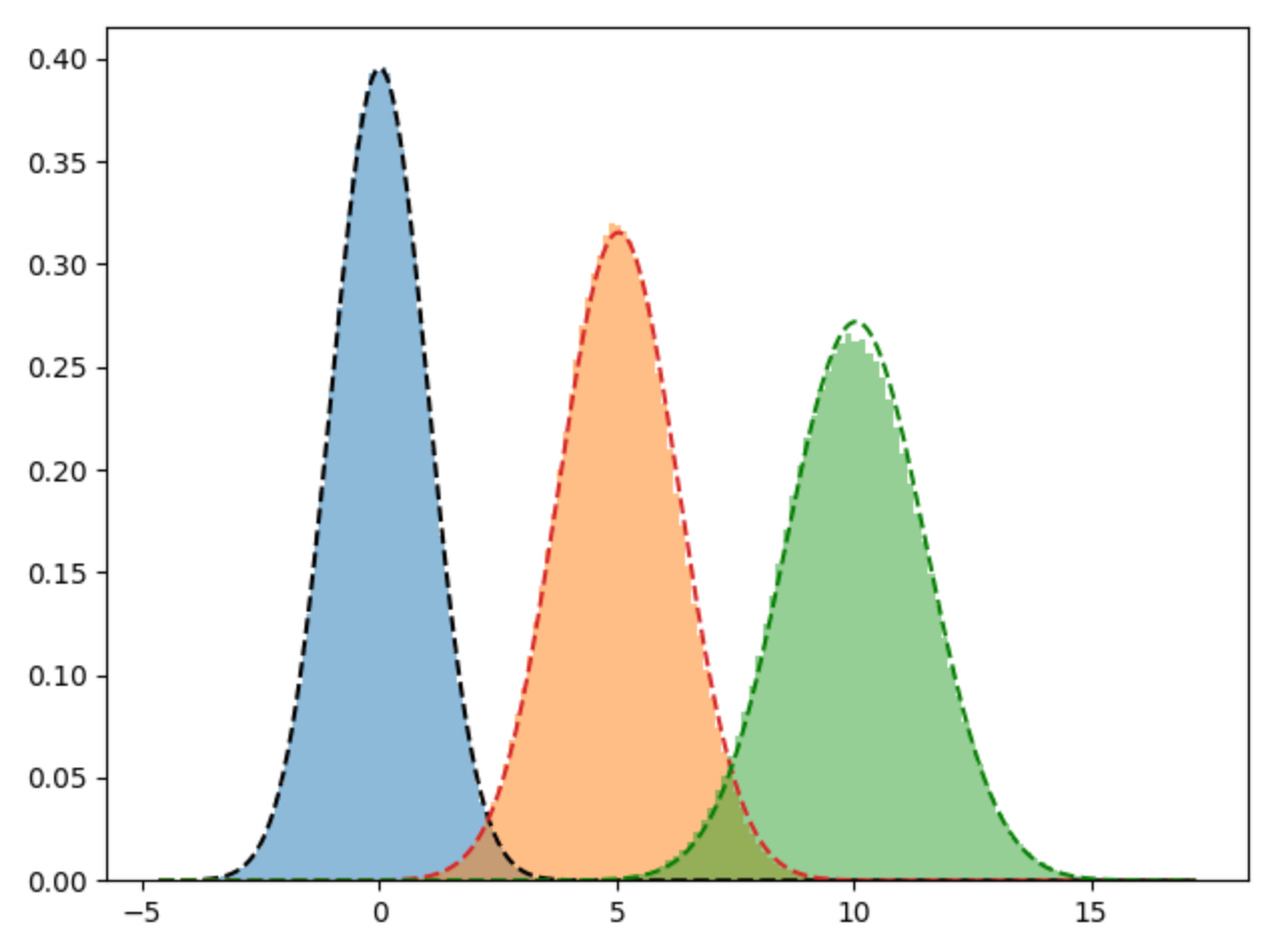
Conclusion
In this post, we covered what latent variables are and how they necessitate the need for an iterative algorithm; that algorithm is the EM algorithm. As an example of the EM algorithm, we implemented a Gaussian Mixture Model in python to show how we can take a dataset and infer the unknown means, and variances of the various gaussian mixtures. Finally, we double check the results of our model to the results of the sklearn gaussian mixture model implementation and found that both models generate similar results.
References
Bishop. (2006). Pattern recognition and machine learning. Springer New York.
Brownlee, J. (2019, November 5). A gentle introduction to maximum likelihood estimation for machine learning. MachineLearningMastery.com. https://machinelearningmastery.com/what-is-maximum-likelihood-estimation-in-machine-learning/
Brownlee, J. (2020, August 27). A gentle introduction to expectation-maximization (EM algorithm). MachineLearningMastery.com. https://machinelearningmastery.com/expectation-maximization-em-algorithm/
Wasserman, L. (2004). All of statistics A concise course in statistical inference Larry Wasserman. Springer.
Wikimedia Foundation. (2024a, April 2). Latent dirichlet allocation. Wikipedia. https://en.wikipedia.org/wiki/Latent_Dirichlet_allocation
Wikimedia Foundation. (2024, September 9). Latent and observable variables. Wikipedia. https://en.wikipedia.org/wiki/Latent_and_observable_variables